Going Deeper • SuperPlotR

Going deeper: advanced SuperPlots

In this vignette, we will explore some of the more advanced features of SuperPlotR.

But first, we need to deal with how to simply scale the plot so it looks good in your paper!

Sizing the SuperPlot

The default setting is to use point sizes of 2 for the data and 3 for the summary points. The font size is 12. This looks good in the RStudio viewer, but is not well suited to a figure which is likely to be very small.

library(SuperPlotR)
# the default plot
superplot(lord_jcb, "Speed", "Treatment", "Replicate", ylab = "Speed (µm/min)")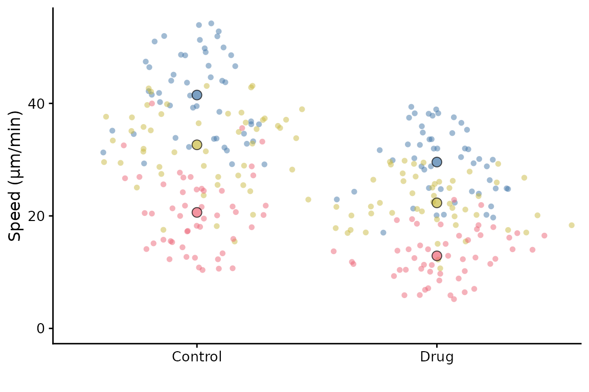

# the same plot but with custom sizing
superplot(lord_jcb, "Speed", "Treatment", "Replicate", ylab = "Speed (µm/min)",
          size = c(0.8,1.5), fsize = 9)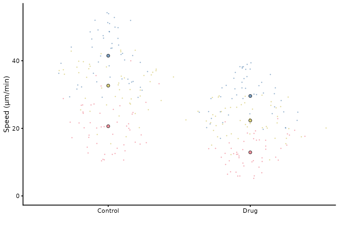

This does not look great in the viewer, but it will look better in a figure.

library(ggplot2)
# the same plot but with custom sizing
superplot(lord_jcb, "Speed", "Treatment", "Replicate",
               ylab = "Speed (µm/min)", size = c(0.8,1.5), fsize = 9)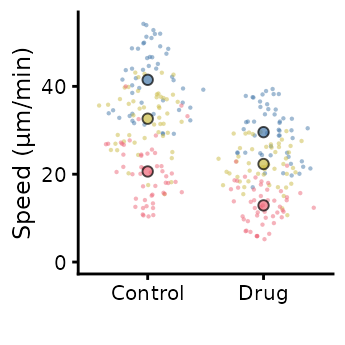

ggsave("plot.pdf", width = 88, height = 50, units = "mm") # final size

This is preferable to

library(ggplot2)
# the same plot but with custom sizing
superplot(lord_jcb, "Speed", "Treatment", "Replicate",
               ylab = "Speed (µm/min)")

ggsave("plot.pdf", width = 88, height = 50, units = "mm") # final size

Customising the SuperPlot

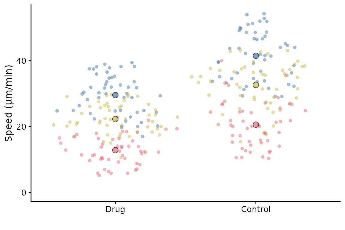
A couple of simple tweaks: an x label can be added, and the transparency of points can be altered like this.

superplot(lord_jcb, "Speed", "Treatment", "Replicate",
          xlab = "Drug", ylab = "Speed (µm/min)", alpha = c(0.3,1))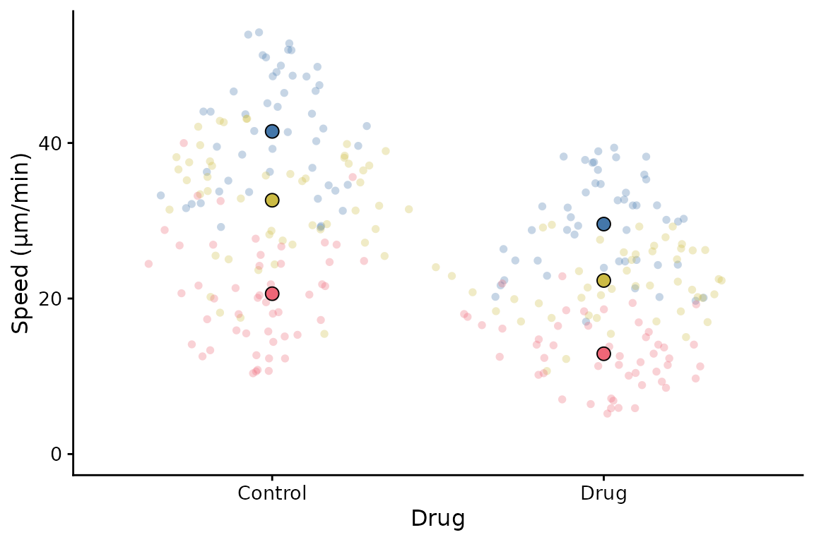

SuperPlotR returns a ggplot object which can be customised how you like. For example, the theme can be overridden like this:

p <- superplot(lord_jcb, "Speed", "Treatment", "Replicate", ylab = "Speed (µm/min)")
p + theme_minimal()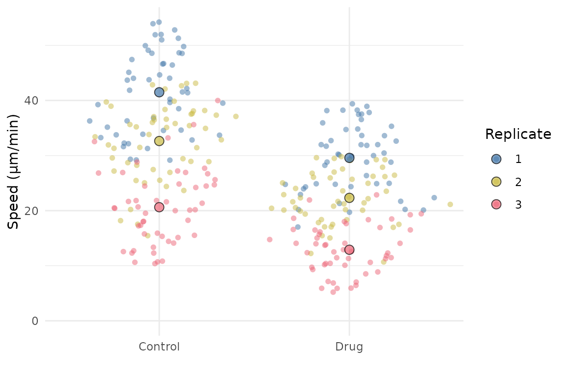

It can also accept a ggplot object using the gg parameter, and then add a SuperPlot to it (within reason!). For example, you might want to plot something behind the SuperPlot.

p <- ggplot() +
  geom_hline(yintercept = 20, linetype = "dashed", col = "grey")
superplot(lord_jcb, "Speed", "Treatment", "Replicate", ylab = "Speed (µm/min)", gg = p)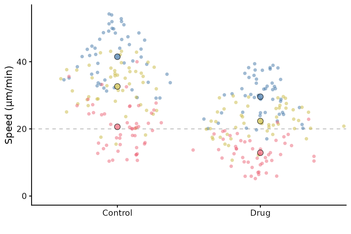

Facetting

Facetting is partially supported. In the simple scenario of facetting by replicate, you can do this:

p <- superplot(lord_jcb, "Speed", "Treatment", "Replicate", ylab = "Speed (µm/min)")
p + facet_wrap(~Replicate)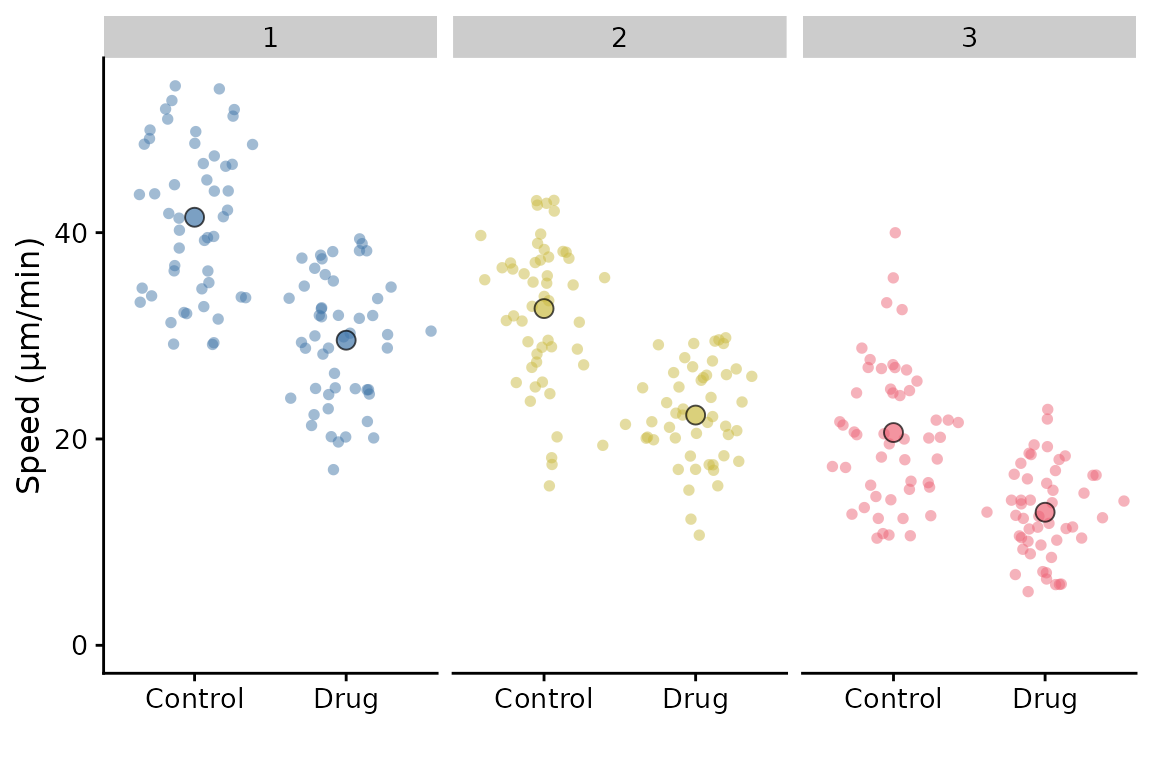

If we had another variable that we wished to facet by, it is possible, but with a limitation: The summary points will remain as the replicate summary and therefore will be the same for each facet. This may not be what you want.

df <- cbind(lord_jcb, other = rep(c("A", "B"), 150))
p <- superplot(df, "Speed", "Treatment", "Replicate", ylab = "Speed (µm/min)")
p + facet_wrap(~other)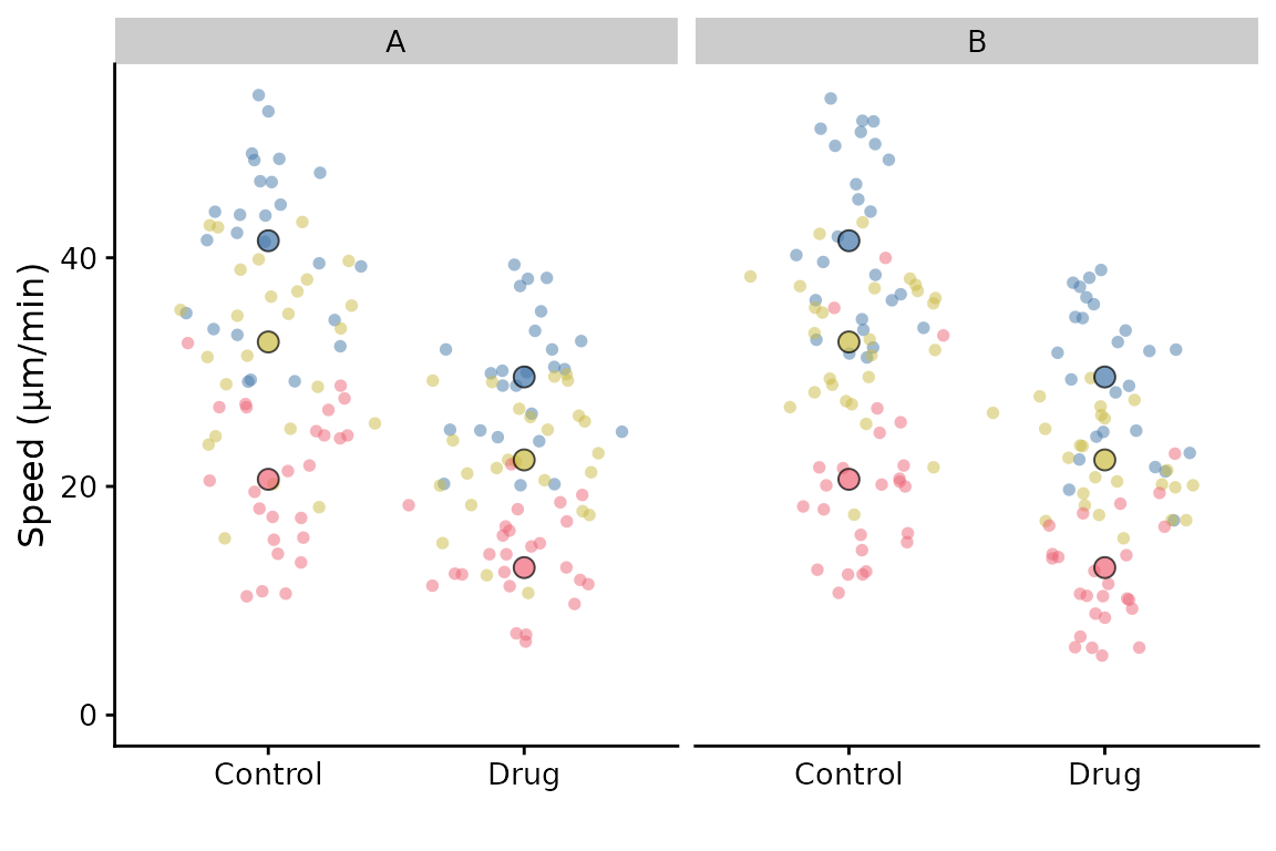

The best way to “facet” like this and have the correct summary points, is to make two superplots after filtering the data for A and B, and then combine them using patchwork or similar package.

Ordering the x-axis

This is best done by reordering the levels of the factor in the input dataframe before calling superplot.

df <- lord_jcb
df$Treatment <- factor(df$Treatment, levels = c("Drug", "Control"))
superplot(df, "Speed", "Treatment", "Replicate", ylab = "Speed (µm/min)")