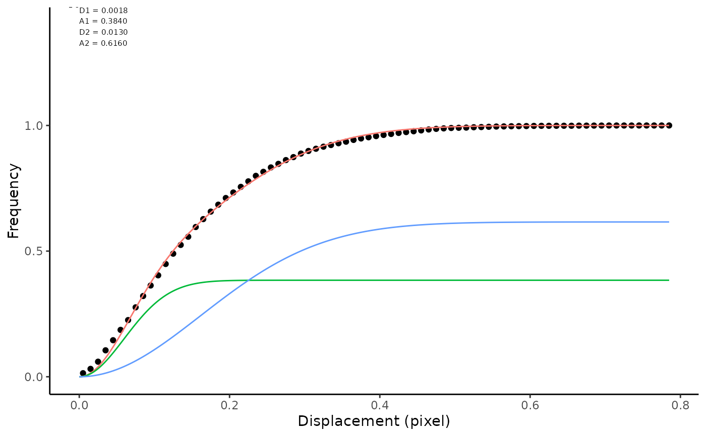
Jump Distances have been calculated for a given time lag. They can be described by fitting curves to the data, either using a histogram or cumulative probability density function. Firtting to a histogram is sensitive to binning parameters and ECDF performs better for general use. The idea behind this analysis is given in: - Weimann et al. (2013) A quantitative comparison of single-dye tracking analysis tools using Monte Carlo simulations. PloS One 8, e64287. - Menssen & Mani (2019) A Jump-Distance-Based Parameter Inference Scheme for Particulate Trajectories, Biophysical Journal, 117: 1, 143-156. This function is called from inside `makeSummaryReport()`, using the defaults. However, you can pass additional arguments for `nPop`, `init` and `breaks` via the ellipsis. Fitting is tricky and two populations (default) is written to catch errors and retry. In the case of failure, try passing better guesses via `init`. To fit 3 populations, you must pass `nPop = 3` as an additional argument, you are advised to also pass guesses via `init`.
Examples
xmlPath <- system.file("extdata", "ExampleTrackMateData.xml", package="TrackMateR")
tmObj <- readTrackMateXML(XMLpath = xmlPath)
#> Units are:  1 pixel and 0.07002736 s
#> Spatial units are in pixels - consider transforming to real units
#> Extracting spot data...
#> Matching track data...
#> Calculating distances...
tmObj <- correctTrackMateData(tmObj, xyscalar = 0.04)
#> Correcting XY scale.
jdObj <- calculateJD(dataList = tmObj, deltaT = 2)
fittingJD(jumpList = jdObj)
#> Warning: All aesthetics have length 1, but the data has 79 rows.
#> ℹ Please consider using `annotate()` or provide this layer with data containing
#>   a single row.
#> Warning: All aesthetics have length 1, but the data has 79 rows.
#> ℹ Please consider using `annotate()` or provide this layer with data containing
#>   a single row.