Make a plot of MSD data — plot_tm

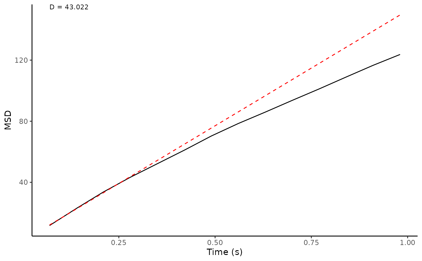
Generate a plot of MSD over a series of increasing time lags. Input is the output from CalculateMSD(), so the plot will display the ensemble or time-averaged MSD (whatever was requested) A fit to the first four points is displayed to evaluate alpha. Diffusion coefficient from this fit is displayed top-left.

plot_tm_MSD(
  df,
  units = c("um", "s"),
  bars = FALSE,
  xlog = FALSE,
  ylog = FALSE,
  auto = FALSE
)

Arguments

df: MSD summary = output from calculateMSD()
units: character vector to describe units (defaults are um, micrometres and s, seconds)
bars: boolean to request error bars (1 x SD)
xlog: boolean to request log10 x axis
ylog: boolean to request log10 y axis
auto: boolean to request plot only, TRUE gives plot and D as a list

Value

ggplot or ggplot and variable

Examples

xmlPath <- system.file("extdata", "ExampleTrackMateData.xml", package="TrackMateR")
datalist <- readTrackMateXML(XMLpath = xmlPath)
#> Units are:  1 pixel and 0.07002736 s 
#> Spatial units are in pixels - consider transforming to real units
#> Collecting spot data. Using 4 cores
#> Matching track data...
#> Calculating distances...
data <-  datalist[[1]]
# use the ensemble method and only look at tracks with more than 8 points
msdobj <- calculateMSD(df = data, method = "ensemble", N = 3, short = 8)
msddf <- msdobj[[1]]
plot_tm_MSD(msddf, bars = FALSE)